4.3 Running the photometry script

The AsPyLib photometry script has been used to reduce a serie of pictures of the asteroid (1036) Ganymed taken on 1st October 2011. We show here the various step of the lightcurve calculation.

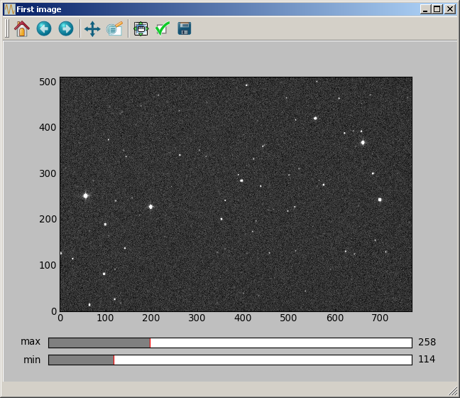
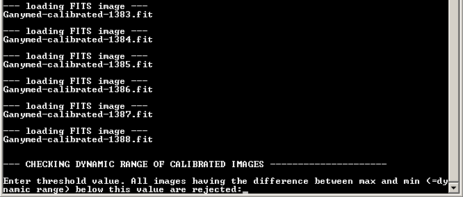
1388 images have been taken during a period of 5h30. Here is the first image in the serie. Ganymed is the bright object on the left of the picture, and it moves rapidly to the right.

Checking input images

The first step that is performed by the script is a carefull check of all input images. First, the dynamic range (as the difference between the max and min values in a certain area of the picture) is computed. The user must decide whether the min and max are calculated over the complete image (option 1) or on a subpart of the image (option 2).

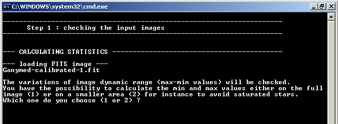
We choose option 1 (typing: 1 + Enter). All pictures are loaded, and after a short time the following curve appears.

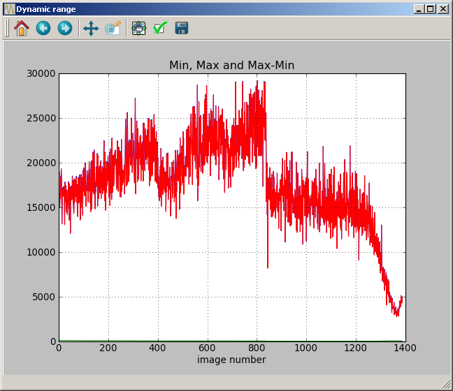
The green curve gives the minimum signal (in that case, close to 0), the blue curve gives the maximum and the red one the difference max-min. In the middle of the night, we see a sudden variation in the amount of measured signal. This difference comes from a change in integration time, which was decided to avoid saturation of Ganymed on the pictures (saturation occurs at 32767 ADU and Ganymed signal was increasing slowly). A few hours later, the signal decreases, due to some fog coming.

The user has the option to remove images with too low signal:

We choose a threshold at 8000 (typing: 8000 + Enter). The images that have been rejected are indicated on the console window:

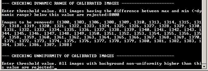
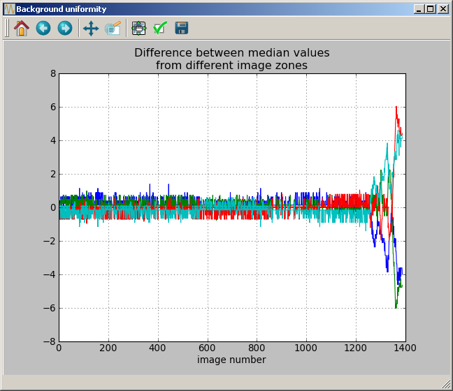
A new curve also appears, that represents the background uniformity. Background uniformity is calculated as the difference between median values in different areas of the image. The curves below show that the uniformity is pretty good. At the end of the night, a slight heterogeneity appears. The user has the possibility to remove images with a too strong nonuniformity.

We choose a threshold at 2 (typing: 2 + Enter). Again, the rejected images are indicated on the console window:

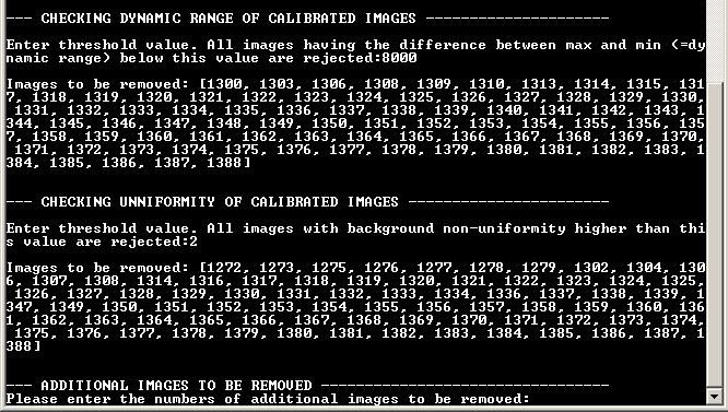
We have now the possibility to reject additional pictures. This can be useful if, for instance, we know that one image in the middle of the night went wrong, due to some bright satellite passing, or to mount vibration, etc. We choose not to reject any image, so we just press “Enter”. Next, the complete list of rejected images appears:

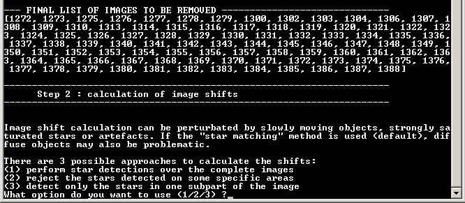
Computing image shifts

The next step is to calculate the shifts of all images in the series with respect to the first image. To do it, we have 3 possibilities. Stars can be detected over the full image (option 1), over the full image except some parts of it (option 2), or over a subpart of the image (option 3).

Since we have a very bright asteroid moving through the complete image it is wise not to choose the option 1, which may fail. So we selection option 3 (typing: 3 + Enter). We are asked to select with the mouse a rectangle in the picture. We do it by right-clicking on the 4 corners of the rectangle. The script calculates the smallest rectangle that encloses the 4 selected positions.

We choose a rectangle that corresponds to the upper right quarter of the image.

Next, the script calculates the image shifts in the series. This step is done separately from the photometry calculation, in order to visualise the complete curve of the (X,Y) shifts and to see immediately if some image shift was wrongly calculated. Then the user can reject these images. After a short time, the plot of the shifts appears:

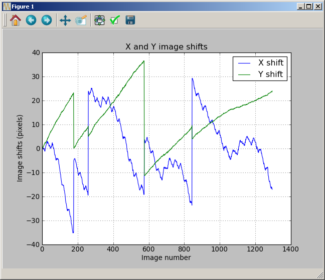
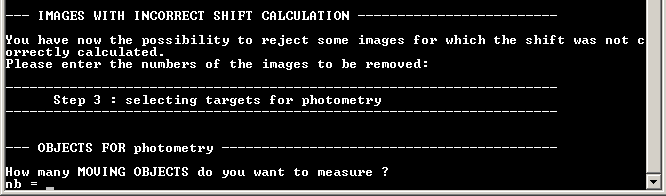
It shows that the image was recentered many times to compensate a too strong drift, but the calculation looks correct. An example of incorrect calculation is shown below:

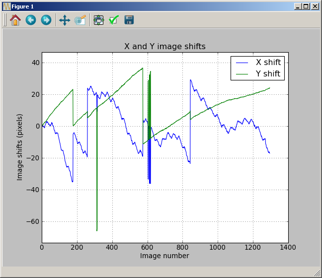
We now have the possibility to reject some images:

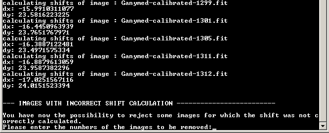
Since the calculation was correct, we just type “Enter”.

Selecting the targets

Next, the user selects the objects for photometry. There are two types of target: asteroids, and variable stars. The user also needs to define reference stars.

We start with the number of asteroids to be measured:

We want to measure one asteroid, so we type: 1 + Enter. Next, we need to select the asteroid on both the first and last images, with a right click. Whenever a selection of objects is made on a picture with AsPyLib, remember two things:

• the left click can be used to zoom in, zoom out, move or go back to initial view of the image
• the right click is only used to select the objects

So there will be only one right click on the first image, and one right click on the last. After the asteroid has been selected, the script is asking for the number of variable stars to be measured. We type: 0 + Enter.

Then we need to select the reference stars. When you don’t know yet how many objects you want to select, you can just enter “-1”:

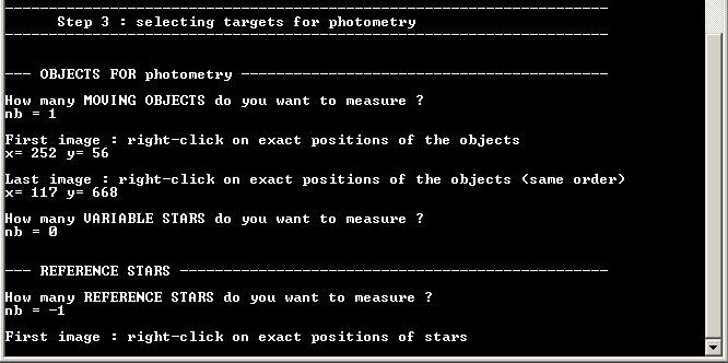
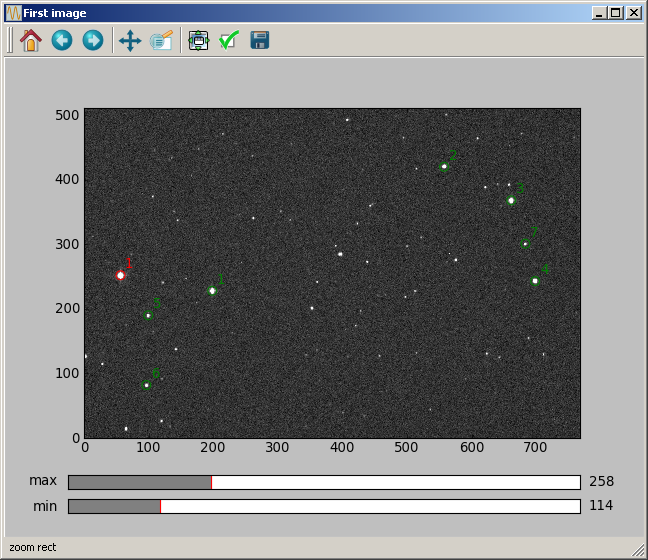
Then it is possible to select as many stars as you want. When there are enough stars selected, you make a right-click in the plotting window but outside of the image to tell the script that you’re done. We have selected 7 reference stars. They are visible below : the asteroid is in red, the reference stars are in green.

Then, the following calculations are made:

• for each object, and for on each image, the script calculates the local maximum (pixel with the maximum signal located in the immediate neighborhood of the selected point)
• for each object, and for on each image, the script makes a fit with a 2D gaussian PSF to calculate the position of the exact centroid
• for each object, each image, each photometry disk size, the photometry is calculated

Checking quality of reference stars

When all this is done, a new plotting window appears, and the user is asked to visually control the quality of the reference stars.

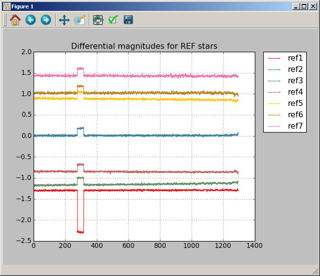
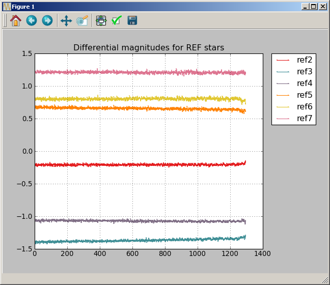
For each reference star, the magnitude curve, minus the average magnitude of all other reference stars, is plotted. The first (so usually the smallest) disk size is used for this computation.

In our case there is a problem with reference star 1. During a short time window, Ganymed comes too close from the star, so that the photometry is no longer done on ref star 1 but on Ganymed ! As a result the magnitude of ref star 1 drops to the magnitude of Ganymed. Actually, Ganymed is not really over ref star 1, but close enough so that the PSF fitting captures Ganymed (brighter) instead of ref star 1 (fainter), and that photometry is made on the wrong target. The curves from the other stars are also impacted, because the represented quantities are the magnitudes of each ref star, minus the average of the magnitudes of the other stars.

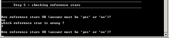
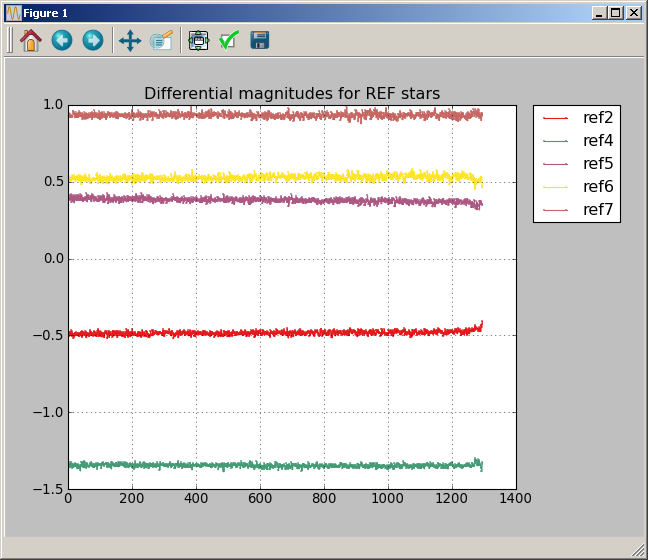
At this point, the user has the choice to remove wrong reference stars. We remove ref star 1 by typing “no” + Enter, and then “1” + Enter and we get:

It’s now much better, but still, reference star 3 is clearly drifting during the night. We remove it by typing “no” + Enter, and then “3” + Enter and we get:

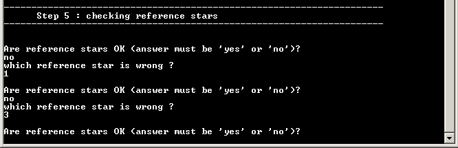
Then we accept the reference stars by typing “yes” + Enter.

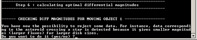
Checking the photometry curves

Finally, the photometry curves obtained with every disk size are displayed. At this point the user has again the possibility to reject some data.

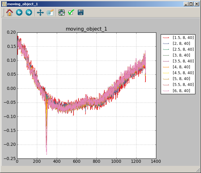
We can see two problems on the above curves. The first problem occurs around image number 300. We can zoom in to try to figure out what went wrong:

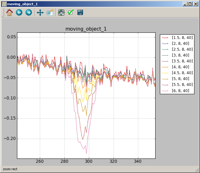
We now see an error which depends on disk size : this is the characteristic signature of the asteroid crossing a star (actually, Ganymed crossing reference star 1). What happens is the following: since Ganymed is brighter than reference star 1, the photometry disk is always well centered on it. But then, due to the close approach some signal coming from reference star 1 comes into the photometry disk. This error is larger for the largest disk sizes, and almost negligible for the smallest disks.

The second problem occurs at the end of the curve. At the end of the observation, there was fog coming and the signal was decreasing. For this reason the measurement may not be very reliable.

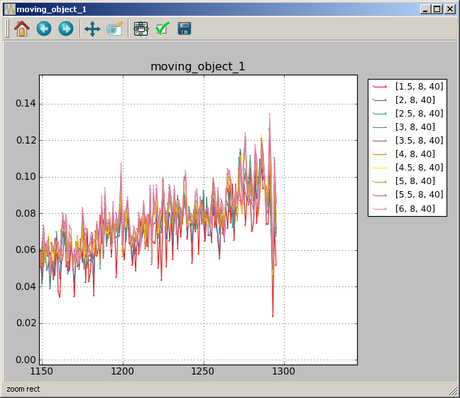
We choosed to keep all photometry disks, and reject two intervals of data: from image 283 to 310 (including 283 and 310) and from image 1292 to 1295 (including 1292 and 1295).

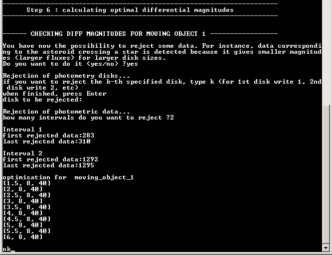
Final results

Once this is done, the script looks for the optimal combinations of disk size, images and reference stars that gives the photometric curves with the smallest noises. For this, the rejected disk sizes, rejected images or rejected reference stars are not considered. If there are P photometry disks and N reference stars that were accepted, then P*(2^N-1) combinations are compared.

Once the best combinations are found, the script has finished its job and you can close the console window by pressing “Enter”.

During the script execution, all the calculated magnitudes and intermediate results (shifts in X and Y, image background uniformity, etc) have been exported to output files:

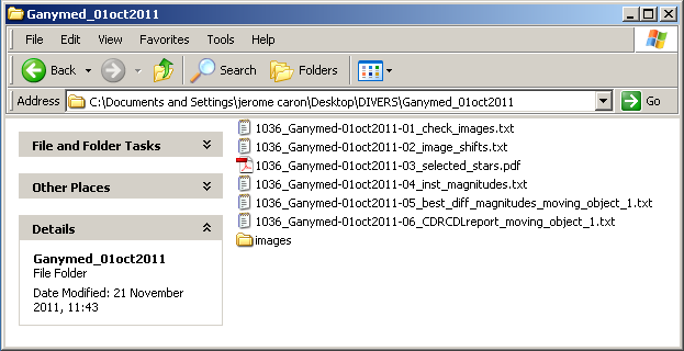
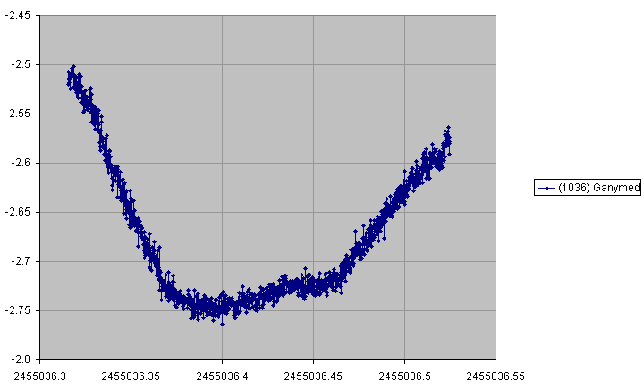
The output file “1036_Ganymed-01oct2011-05_best_diff_magnitudes_moving_object_1.txt” can be opened with Excel. It contains the 10 best magnitude curves. The first one can be plotted with Excel: